
LiDAR-in-the-loop Hyperparameter Optimization
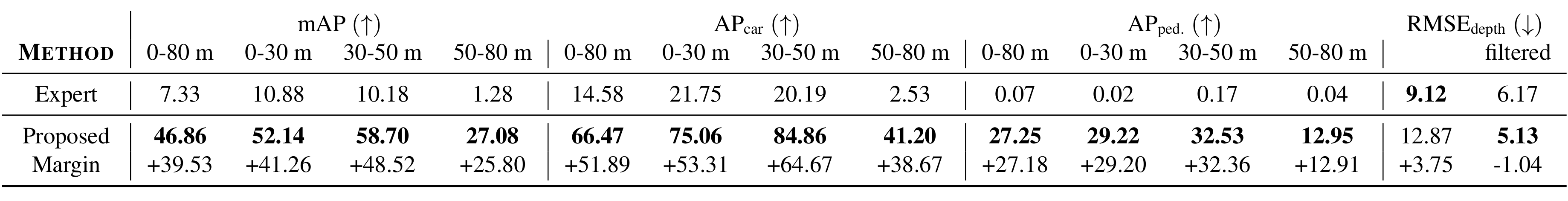
End-to-end optimization of a LiDAR pipeline (LiDAR unit and DSP) results. LiDAR and DSP simulated with an extension of the traffic simulator CARLA. Left: Rendering of the scene as seen by a forward facing virtual camera. The remaining renderings show LiDAR Point Clouds color-coded with returned beam intensity, and bounding boxes of cars and pedestrians. Second from left: ground truth. Third from left: Expert-tuned LiDAR and DSP. Last: LiDAR and DSP optimized with the proposed method. Optimization results in clutter-free point clouds which trigger fewer false positive detections. For visualization purposes only the camera field-of-view is shown.
LiDAR has become a cornerstone sensing modality for 3D vision. LiDAR systems emit pulses of light into the scene, measure the returned signal, and rely on hardware digital signal processing (DSP) pipelines to construct 3D point clouds from the measurements. Point clouds produced by LiDAR DSPs are input to downstream 3D vision models – as training datasets and at inference time. Existing LiDAR DSPs are composed of cascades of parameterized operations; modifying configuration hyperparameters results in significant changes in the point clouds and consequently the output of downstream methods. Existing methods treat LiDAR systems as fixed black boxes and construct downstream task networks more robust with respect to measurement fluctuations. Departing from this approach, the proposed method directly optimizes LiDAR sensing and DSP hyperparameters for downstream tasks. To investigate the optimization of LiDAR system hyperparameters, we devise a realistic LiDAR simulation method that generates raw waveforms input to a LiDAR DSP. We optimize LiDAR hyperparameters for both 3D object detection IoU losses and depth error metrics by solving a nonlinear multi-objective optimization problem with a 0th-order stochastic algorithm. For automotive 3D object detection models, the proposed method outperforms manual expert tuning by 39.5% mean Average Precision (mAP).
LiDAR-in-the-loop Hyperparameter Optimization
LiDAR-in-the-loop Hyperparameter Optimization
Félix Goudreault, Dominik Scheuble, Mario Bijelic, Nicolas Robidoux, Felix Heide
CVPR 2023
Optimization Algorithm
LiDAR hyperparameter optimization was performed with a variant of the Covariance Matrix Adaptation-Evolution Strategy (CMA-ES) optimization method, with a champion selection criterion based on the stable dynamic max-rank loss scalarization, also used to drive optimization. The champion converges to a Pareto-optimal solution which balances the different objectives whereas most Multi-Objective Optimization algorithms are not designed to converge to a specific optimal solution.
Point cloud depth and intensity optimization using proposed algorithm. Top left: Point cloud obtained with the configuration sampled by the optimizer at each step. Bottom left: Point cloud obtained with the hyperparameter values of each step's champion. Point cloud color encodes depth error (clipped at 1m); lighter is better. Top right: Depth and intensity RMSE for each step's sampled LiDAR configuration (in blue; top is depth RMSE, bottom is intensity RMSE), with each step's champion depth and intensity RMSE (in orange; red star marks champion), and approximate Pareto front (green dots). Bottom right: Pareto front approximation found at each step (green dots) with champion highlighted (red star), with the true Pareto front, computed by aggregating multiple optimization runs, shown in gray.
LiDAR-in-the-loop Optimized Depth and Intensity
LiDAR units reconstruct depth and reflected light intensities from sampled waveforms. We show simulated point clouds for a realistic 3D scene animated by the CARLA engine. We compare the reconstruction errors of the optimal solution obtained with the proposed multi-objective optimization method with those obtained by manual expert-tuning. The depth error of each cloud point is color-coded: darker means a higher error. Compared to optimized point clouds, expert-tuned point clouds suffer from clutter, with depth errors that increase with distance.
LiDAR-in-the-loop Optimized Object Detection
We validate our optimization method on an automotive detection and classification task by adding car and pedestrian detection AP as new objectives to be optimized along depth and intensity reconstruction errors (see video at top of page). The following table contains a quantitative comparison between the proposed method and expert tuning. Compared to manual expert tuning, the proposed method increases AP by 51.89% for cars and 27.18% for pedestrians, on the full 0-80m range, with large increases predominately at close range. We also compare the average depth RMSE before and after filtering suppressed points; the low loss of the filtered point cloud suggests that clutter has been removed and that the detector prefers an accurate if sparser point cloud. Note however that a DSP optimized for the removal of clutter, like the proposed method, also suppresses ground points, with a small impact on object detection results (see the last column).
Simulation
Commercial LiDAR units are IP-protected black boxes with very limited hyperparameter access. In order to assess our optimization method, we introduced a LiDAR model that plugs into the CARLA traffic simulation environment. The proposed model computes the full transient noisy waveform formed by multiple laser echoes. In addition, the model provides a set of hyperparameters that controls the operations of the LiDAR unit and the subsequent DSP model.
LiDAR Simulation Model
We propose a parameterizable LiDAR simulation model, based on the CARLA traffic simulation engine, that generates full transient waveforms by extracting scene response, ambient light and object reflectances. First, we build a Bidirectional Reflectance Distribution Function (BRDF) for simulated laser beams using material properties extracted from custom shaders. Then, we sample the simulated environment using ray casts from which we construct single-peak waveforms using the BRDF and pulse characteristics. After adding the ambient light extracted from a full rendering of the scene, we simulate multi-path effects by downsampling adjacent rays into a single wavefront which is then processed by the DSP after the addition of noise. The point cloud returned by the DSP is fed to an object detector. The resulting APs, together with other point cloud quality metrics, are passed to the proposed optimization algorithm which suggests new LiDAR and DSP configuration hyperparameter values to test. This closes the optimizing loop. In this model, both the beam configuration and the DSP hyperparameters influence the output point cloud; they are simultaneously optimized.
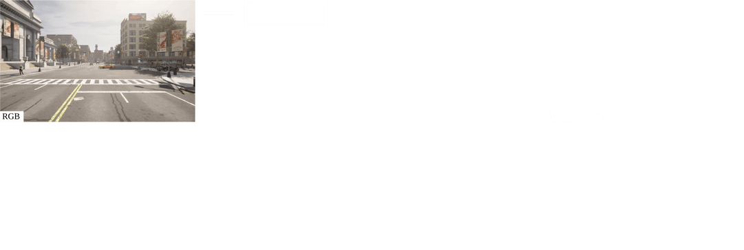
LiDAR Sensing and DSP ModelThe DSP model converts raw waveforms to a 3D point cloud that contains range and intensity information. LiDAR sensing and DSP hyperparameters, e.g., pulse power, pulse duration and noise floor, can be set for every LiDAR channel independently. Changing the values of the hyperparameters strongly and nonlinearly changes the output point cloud. Our DSP model is depicted on the figure on the right and includes denoising, ambient light estimation, rising edge detection and intensity estimation. |
 |
Off-the-shelf LiDAR Optimization
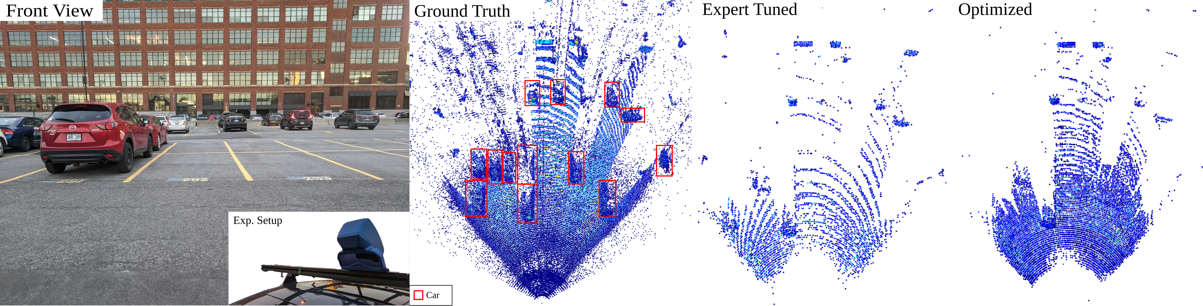
We validate our proposed approach with an off-the-shelf LiDAR sensor. Only a handful of hyperparameters are user-accessible. Because raw waveforms are inaccessible, we optimize 3D point cloud histograms taken over an (intermittently) static scene such as a workplace parking lot. The ground truth histogram, shown on the 2nd panel, was generated by averaging captures with a uniform angular resolution scanning pattern. Expert-tuned, resp. optimized, contributions to the histograms from which the loss driving the optimization is computed are shown in the 3rd, resp. last, panel where darker blue means better. Optimized hyperparameters achieved better results by focusing laser scans in regions of interests (ROIs) where the ground truth was denser. We estimate a 10.1 cm error for the expert-tuned configuration vs. 3.0 cm with optimized hyperparameters. A picture of the front view scene is shown on the leftmost panel.
Related Publications
[1] Ethan Tseng, Ali Mosleh, Fahim Mannan, Karl St. Arnaud, Avinash Sharma, Yifan Peng, Alexander Braun, Derek Nowrouzezahrai, Jean-François Lalonde, Felix Heide. Differentiable Compound Optics and Processing Pipeline Optimization for End-to-end Camera Design. SIGGRAPH 2021
[2] Ali Mosleh, Avinash Sharma, Emmanuel Onzon, Fahim Mannan, Nicolas Robidoux and Felix Heide. Hardware-in-the-Loop End-to-End Optimization of Camera Image Processing Pipelines. CVPR 2020
[3] Nicolas Robidoux, Luis E. Garcia Capel, Dong-eun Seo, Avinash Sharma, Federico Ariza and Felix Heide. End-to-End High Dynamic Range Camera Pipeline Optimization. CVPR 2021